Although this is a relatively new branch of science that developed over the last 15 years, there are many groups that compute these connections. Our approach in the World Weather Attribution (WWA) collaboration is different in two ways: we attempt to have our results ready as soon as possible after the event, and we try to respond as much as possible to questions posed by the outside world. Both approaches aim to make the attribution studies more useful. Commissions to investigate a disaster typically operate within a few months and appreciate if the event being attributed is as close as possible to the aspects that caused the disaster, media interest that reaches a large audience wanes on the order of weeks to months after large events.
We started doing event attributions on our first physical meeting during a heat wave in Paris in the summer of 2015 and learned a lot of lessons from the over two dozen studies we performed since then. These are summarised in a scientific paper that was published in April 2021, Pathways and pitfalls in extreme event attribution. This article is a summary of the scientific paper. An even more detailed description of the methodology that resulted from all these lessons learned has been published as A protocol for probabilistic extreme event attribution analyses. The main lesson was that the actual attribution step, on which most attention was focused in 2015, was only one step out of eight. We needed ways to deal with:
- the trigger: which studies to perform,
- the event definition: which aspect of the extreme event were most relevant,
- observational trend analysis: how rare was it and how has that changed,
- climate model evaluation: which models can represent the extreme,
- climate model analysis: what part of the change is due to climate change,
- hazard synthesis: combine the observational and model information,
- analysis of trends in vulnerability and exposure, and
- communication of the results.
We discuss each step in turn.
1. Analysis trigger
The Earth is large and extreme weather occurs somewhere almost every day. Which of these events merit an attribution study? In WWA we try to prioritise events that have a large impact on society, or that provoked a strong discussion in society, so that the answers will be useful for a large audience. These are often events for which the Red Cross issues international appeals. Sometimes smaller events closer to home or even meteorological records that did not affect many people also seem to generate enough interest to spend the effort to obtain a scientifically valid answer to the attribution question. We explicitly do not include the expected influence of climate change on the event on the trigger criteria: the result that an event was not affected by climate change, or even became less likely, is just as useful as one that the probability increased.
2. Event definition
Defining the event turned out to be both much harder and more important than we thought when we started attribution science. As an example: the first published extreme event attribution study analysed the extremely hot summer of 2003 in Europe (Stott et al, 2004). It took as event definition a European-wide seasonally averaged temperature, whereas the impacts had been tens of thousands of deaths in the 10-day hottest period in cities. A large-scale event definition like a continental and seasonal average has the advantage that climate models can represent it better and the signal-to-noise ratio is usually better than a local, short time scale definition. However, it is not the event that caused the damage and in WWA we try to relate our attribution question to the impacts, so we usually choose a definition of the event that corresponds as closely as possible to the impacts.
However, we stick to meteorological or hydrological quantities, like temperature, wet bulb temperature, rainfall, river discharge and do not consider real impacts like number of deaths or economic damage. The reason is that the translation from extreme weather into impacts usually is a complex and uncertain function of the weather. It also changes over time: the introduction of heat plans in Europe after the disastrous heat waves of 2003 and 2006 has reduced the number of deaths per degree of heat by a factor of two or three. Similarly, more houses in natural areas have increased the risk of wildfire damage, or more houses on the coast are now exposed to storm damage. We do not have the expertise to also take these changes into account and therefore restrict ourselves to indicators of heat, fire weather risk and wind in these examples.
A final consideration of the choice of event definition is that the quantity chosen has to have long and reliable observations and be represented by climate models.
In practice we use the following definitions. For heat waves, the local highest daily maximum temperature of the year is a standard measure that captures the health risk to outdoor labourers in e.g. India. For Europe and North America, the maximum of 3-day mean temperature appears to be more relevant as the most vulnerable population is indoors. If humidity plays a role the wet bulb temperature can be used instead. For cold waves we just use temperature as the wind chill is hard to measure. Local daily maximum precipitation is usually relevant for flash floods, for larger floods we either average over a river basin or use hydrological models to compute river discharge. Drought has many definitions, from lack of rain to water shortage and great care has to be taken to choose the most relevant one. For wind the highest 10-minute or hourly wind speed is chosen as these are closest to the impacts.
It should be noted that in practice, finding out what really happened is not easy as different estimates of the variable can be very different. An example is given in Fig. 1, which shows the very different estimates of the highest 3-day averaged precipitation around Houston due to Hurricane Harvey from different observing systems. We used the GHCN-D station data.
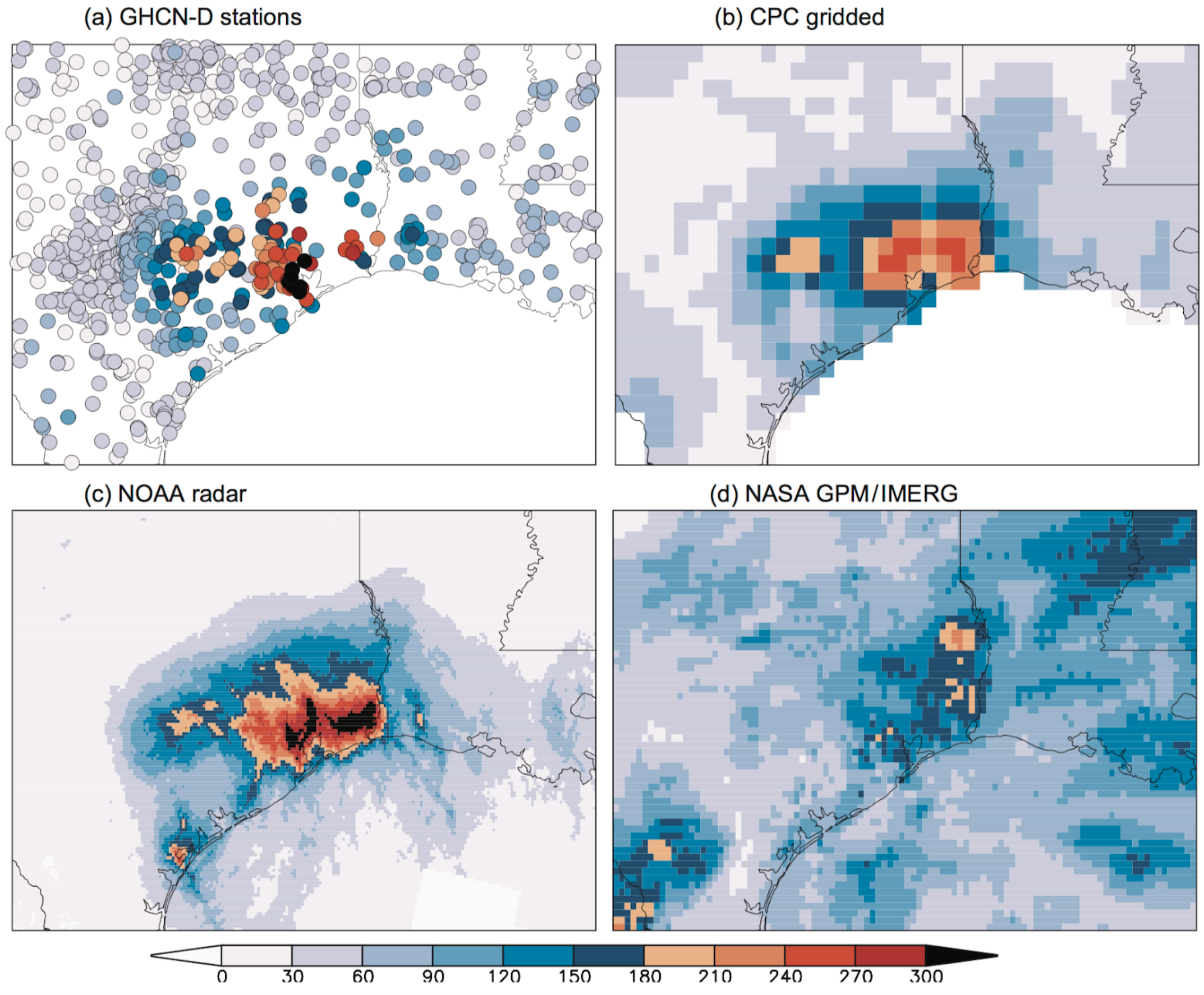
Figure 1: Observed maximum three-day averaged rainfall over coastal Texas January-September 2017 (mm/dy). a) GHCN-D v2 rain gauges, b) CPC 25 km analysis, c) NOAA calibrated radar (maximum in August 25–30), d) NASA GPM/IMERG satellite analysis. From Van Oldenborgh et al. (2017).
3. Observational trend analysis
In WWA, we consider an analysis of the observations an essential part of an extreme event attribution. The observational dataset should go back at least to the 1950s but preferably to the 19th century and be as homogeneous as possible. To choose the most representative observation we usually collaborate with local experts, who know which time series are most reliable and least influenced by other factors than climate change, e.g., station changes, irrigation or urban heat.
The observational analysis gives two pieces of information: how rare the event is in the current climate and how much this has changed over the period with observations.
The probability in the current climate is very important to inform policy makers whether this is the kind of event that you should be able to handle or not. As an example, the floods that paralysed Jakarta in January 2014 turned out to be caused by a precipitation event with a return times of only 4 to 13 years, pointing to a very high vulnerability to flooding (which is well-known). Conversely, the floods in Chennai in December 2015 were caused by rainfall with an estimated return period of 600 to 2500 years, which implies that the event was too rare to make it worth it to defend against.
Climate change is by now so strong that many observed time series of extreme events show clear trends. An efficient way to quantify the changes is to fit the data to an extreme value distribution, which theoretically describes either block maxima like the hottest day of the year, or exceedances over a threshold like the 20% driest years. We describe the effects of climate change by either shifting or scaling the distribution with the 4-yr smoothed global mean surface temperature (GMST). This quantity is proportional to the anthropogenic forcing and estimates are available in real time. The smoothing serves to remove influences of El Niño and other weather that are unrelated to the long-term trends. The assumptions in these fits—constant variability for temperature, constant variability over mean for precipitation and other positive-definite quantities—can be checked in the observations themselves to some extent and more fully in the climate model output.
In practice we find that there are very clear trends in heat waves, although these are also influenced strongly by non-climatic factors such as land use changes, irrigation and air pollution. Cold waves also show significant trends by now, although due to the greater variability of winter weather the signal-to-noise ratio is not as good as for heat waves. Daily or sub-daily precipitation extremes also often show clear trends, longer-duration ones are more mixed. Drought trends are very difficult to see in observations, because droughts are long-term phenomena so there are not many independent samples. Drought is also usually only a problem when the anomaly is large relative to the mean, which usually implies that it is also large relative to the trend, so the signal-to-noise ratio is poor. In all our drought studies only one showed a borderline significant trend in precipitation.
Fig. 2 shows the trend in a heat extreme (the highest daily mean temperature at De Bilt, the Netherlands), which shows a clear trend by eye already, and 3-day precipitation extremes along the US Gulf Coast, for which the GEV fit shows a significant trend under the assumption that all intensities increase by the same percentage.
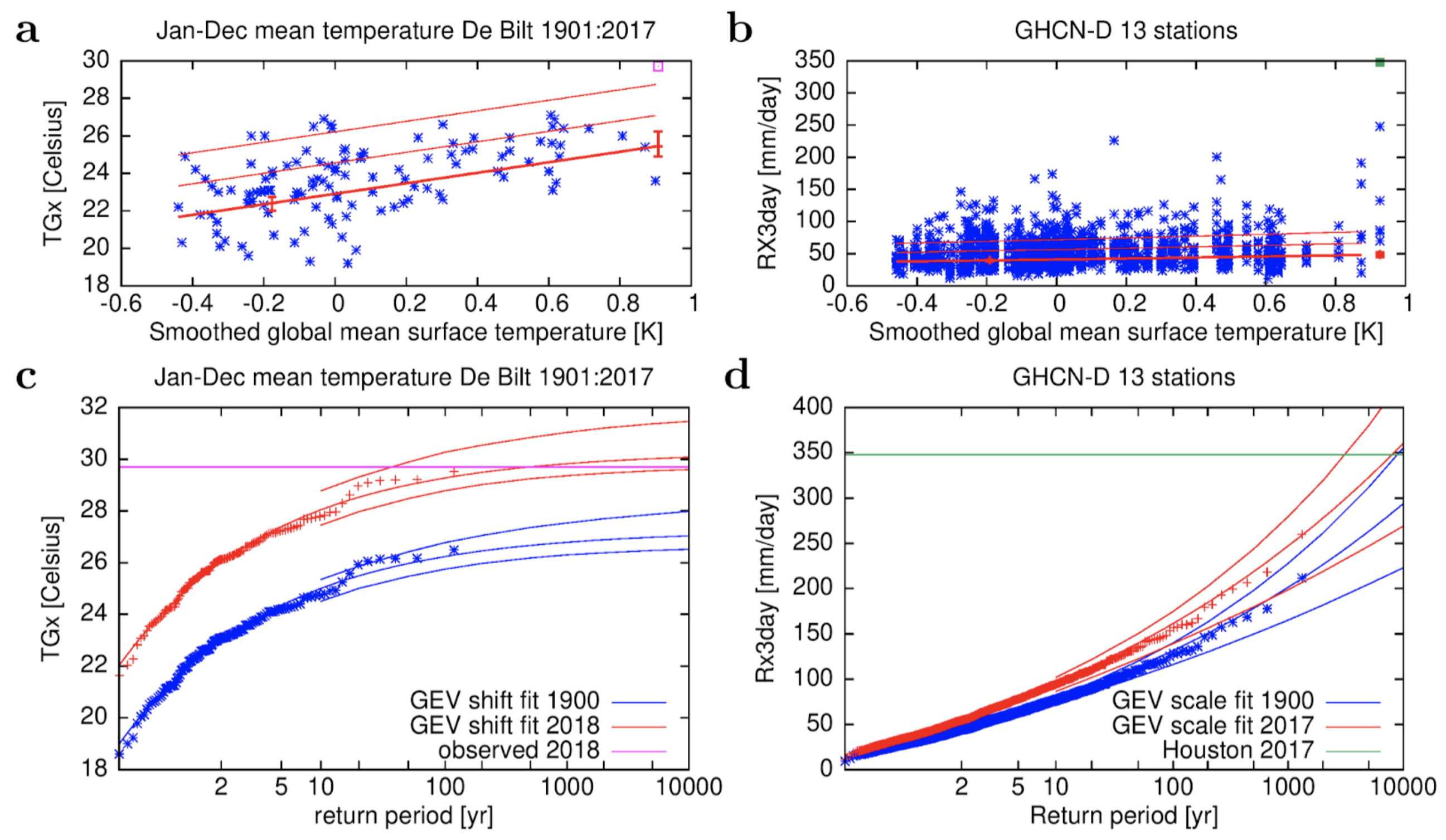
Figure 2: a,c) Highest daily mean temperature of the year at De Bilt, the Netherlands (ho- mogenised) for the period 1901-2018, fitted to a GEV that shifts with the 4-yr smoothed GMST. a) as a function of GMST and c) in the climates of 1900 and 2018. b,d) The same for the highest 3-day averaged precipitation along the US Gulf Coast for 13 stations with at least 80 years of data and 2º apart, fitted to a GEV that scales with 4-yr smoothed GMST. From climexp.knmi.nl, (b,d) also from Van Oldenborgh et al. (2017).
4. Climate model evaluation
Observations alone cannot show what caused the trend. In order to attribute the observed trend to global warming (or not), we have to use climate models. These are similar to the weather models that we use to forecast the weather of the next days to weeks, but instead of predicting the specific weather the next few days, they predict the statistics of it: how often extreme events occur in the computed weather in the climate model. However, we can only use the climate model output if these extremes are realistically simulated. In practice we use the following three criteria to select an ensemble of climate models.
- Can the model represent the extreme in principle?
- Is the statistical distribution of extreme events on the climate model compatible with the observed one, allowing for a bias correction?
- Is the meteorology leading to these extremes in the model similar to the observations?
The first criterion usually concerns the resolution and included mechanisms. A relatively coarse resolution model with a 200 km grid may well be able to represent a heat wave, but for somewhat realistic tropical cyclones we need a resolution better than 50 km. If we study heat in an area where irrigation is important we would like the model to include that cooling influence on extreme temperatures.
For the second criterion we just fit the tail of the distribution to the same extreme value function as the observations and check whether the variability and shape of the tail are compatible. To verify that the agreement is not for the wrong reasons we try to check the meteorology behind the extremes. This includes in any case the seasonal cycle and spatial patterns, but if relevant also may concern El Niño teleconnections or the source of precipitation. We even found that many climate models have an unphysical limit on high precipitation amounts (Fig. 3), these cannot be used for attributing (or projecting) these kind of events.
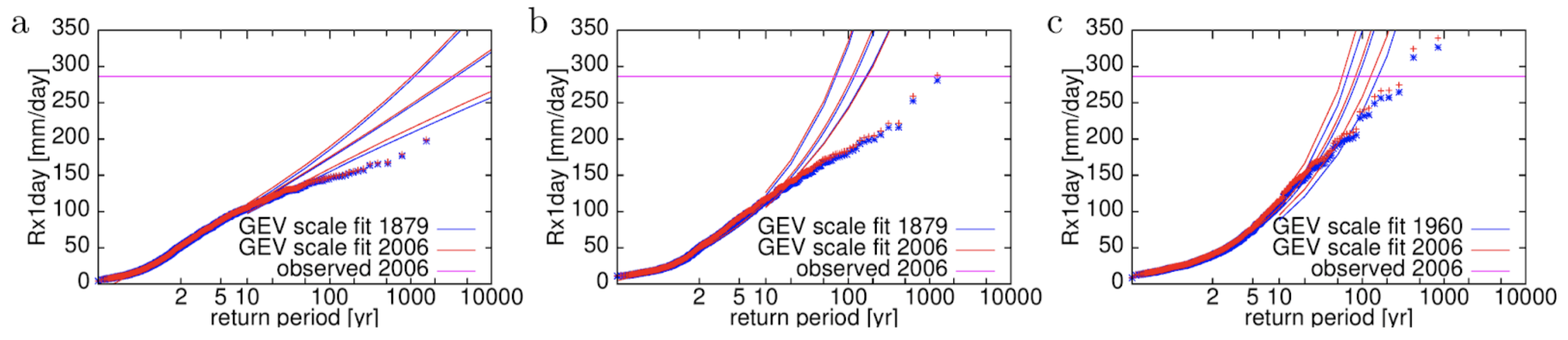
Figure 3: Return time plots of extreme rainfall in Chennai, India, in two CMIP5 climate models with ten ensemble members (CSIRO-Mk3.6.0 and CNRM-CM5) and an attribution model (HadGEM3-A N216) showing an unphysical cut-off in precipitation extremes. The horizontal line represents the city-wide average in Chennai on 1 December 2015 (van Oldenborgh et al., 2016)
As climate models are imperfect representations of reality we demand at least two and preferably more models to be good enough for the attribution analysis. The spread of these models gives an indication of the model uncertainty.
5. Climate model analysis
The next step is the original attribution step. For each model we compute how much more likely or intense the extreme event has become due to anthropogenic emissions of greenhouse gases and aerosols. This can be done in one of two ways. The original proposal was to simulate the world twice: once for the current climate and once for a counterfactual climate that is the same as the current one but without anthropogenic modifications of the climate. For each climate we perform many simulations of the weather and count or fit the number of extremes. The difference between the two gives how much more (or less) likely the extremes have become.
The alternative is to take simulations of the historical climate, usually extended with a few years of the climate under one of the climate scenarios up to the current year (these are very close together up to 2040 or so). These transient simulations can then be analysed exactly the same way as the observations. This assumes that the influence of natural forcings—variations in solar radiation and volcanic eruptions—is small compared to the anthropogenic ones, which is usually the case.
As climate models usually have biases, we define the event by its return period and not by its amplitude. So if the observational analysis gives a return period of 100 yr, we also count or fit 100-yr events in the models. This turns out to give a better correspondence to the observations than specifying the amplitude and explicitly performing a bias correction when the extreme value distribution has an upper bound, as usually occurs for heat extremes, or a very thick tail, which we find for precipitation extremes.
For each model the attribution step gives a change in probability for the extreme to occur due to anthropogenic climate change, or equivalently the change in intensity for a given intensity.
6. Hazard synthesis
The next step is to combine the information from the observations and multiple models into a statement how the probability and intensity of the physical extreme event has changed. We use the term ‘hazard’ for this as the total ‘risk’ also includes how much exposure there is to the extreme and how vulnerable the people or systems are, which is addressed in the next step.
How to best combine this information is still an area of active research. Our current method is to combine all observational estimates under the assumption that they are highly correlated, as they are based on the same observations of the same sequence of weather. The model estimates are combined under the assumption that they are not correlated, as the weather in each model is different. However, the model spread can be larger than expected on the basis of weather variability alone, in which case we add a model uncertainty term to the average. Finally we combine observations and models. If they agree this can be a weighted average, but if they disagree we either have to increase the uncertainty or even give up on an attribution altogether.
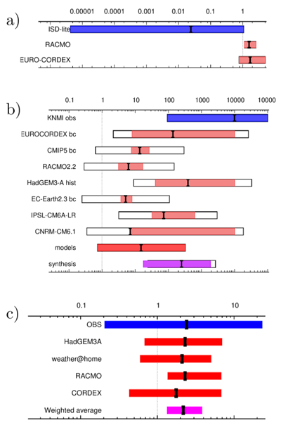
Figure 4: Synthesis plots of a) the probability ratio (PR) for changes in wind intensity over the region of storm Friederike on 18 January 2018 (Vautard et al., 2019), b) the PR for the highest 3-day averaged daily mean temperature of the year at De Bilt, the Netherlands (Vautard et al, 2020) and c) the PR for extreme 3-day averaged precipitation in April–June averaged over the Seine basin (Philip et al., 2018a). Observations are shown in blue, models in red and the average in purple. An additional model uncertainty term is added as black outline boxes.
An example of the latter is our study into the winter storms that hit Europe in January 2018, Fig. 4a. The climate models compute a small increase in probability due to the increased temperature, but the observations show a large decrease. We think the latter is caused by the increased roughness of the land surface due to more buildings, trees and even wind turbines. This is not included in the climate models, so they cannot be expected to give a reliable projection of the intensity of future storms.
A less severe discrepancy is apparent in heatwaves in northwestern Europe, Fig. 4b. The models simulate a much lower trend than the observations. This means we can only give lower bounds on the changes in probability and intensity due to human induced climate change. The same holds for southeastern Australia.
In other studies observations and models agree well and we can give an accurate attribution statement based on the combination of all information, e.g. for the rainfall in the Seine basin in 2016 (Fig. 4c).
7. Vulnerability and exposure
A disaster happens due to a combination of three factors:
- the hydrometeorological hazard: process or phenomenon of atmospheric, hydrological or oceanographic nature that may cause loss of life, injury or other health impacts, property damage, loss of livelihoods and services, social and economic disruption, or environmental damage,
- the exposure: people, property, systems, or other elements present in hazard zones that are thereby subject to potential losses, and
- the vulnerability: the characteristics and circumstances of a community, system or asset that make it susceptible to the damaging effects of a hazard.
We consider it essential to also discuss the vulnerability and exposure in an attribution study. Not only do these combine with the changes in the physical extremes that we have computed in the previous step to determine the impact of the extreme weather, but they may have significant trends themselves.
As an example: we found that the drought in São Paulo, Brazil in 2014–2015 was not made worse due to climate change. Instead, the analysis showed that the increase of population of the city by roughly 20% in 20 years, and the even faster increase in per capita water usage, had not been addressed by commensurate updates in the storage and supply systems. Hence, in this case, the trends in vulnerability and exposure were the main driver of the significant water shortages in the city.
Even though this section often has to be qualitative due to a lack of standardised data and literature describing trends in these factors, we think it is vitally important to put the extreme weather into the perspective of how it impacts society or other systems. Changing the exposure or vulnerability is also often the way to protect against similar impacts in the near future, as stopping climate change is a long-term project and we expect in general stronger impacts over the next decades. For instance the number of casualties of heat waves has decreased by a factor two or three in Europe after heat plans were developed in response to the 2003 and 2006 heat waves. Similar approaches are now being taken throughout the world. The inclusion of vulnerability and exposure is thus vital to making the analysis relevant for climate adaptation planning.
8. Communication
Finally, the results of the attribution study have to be communicated effectively to a range of audiences. We found that the key audiences that are interested in our attribution results should be stratified according to their level of expertise: scientists, policy-makers and emergency management agencies, media outlets and the general public.
For the scientific community a focus on allowing full reproducibility is key. We always publish a scientific report that documents the attribution study in sufficient detail for another scientist to be able to reproduce or replicate the study’s results. If there are novel elements to the analysis the paper should also undergo peer review. We have found that this documentation is also essential to ensure consistency within the team on numbers and conclusions.
We have found it very useful to summarise the main findings and graphs of the attribution study into a two-page scientific summary aimed at science-literate audiences who prefer a snapshot of the results. Such audiences include communication experts associated with the study, science journalists and other scientists seeking a brief summary.
For policy-makers, humanitarian aid workers and other non-scientific professional audiences, we found that the most effective way to communicate attribution findings in written form are briefing notes that summarise the most salient points from the physical science analysis and the specific vulnerability and exposure context. This audience often requires the information to be available relatively quickly after the event.
Finally, if there is a demand from the media, a press release with the main points and quotes from the study leads and local experts is prepared. In addition to the physical science findings, these press releases typically provide a very brief, objective description of the non-physical science factors that contributed to the event. In developing this press piece, study authors need to be as unbiased as possible, for instance not emphasising lower bounds as conservative results because in practice this may lead to interpretations that underestimate the influence of climate change. This is also an effective way to reach other target audiences.
Conclusions
Using the procedure outlined above, based on lessons learned during five years of doing attribution studies, we found that often, we could find a consistent message from the attribution study based on imperfect observations and model simulations. This we used to inform key audiences with a solid scientific result, in many cases quite quickly after the event when the interest is often highest.
However, we also found many cases where the quality of the available observations or models was just not good enough to be able to make a statement on the influence of climate change on the event under study. This also points to scientific questions on the reliability of projections for these events and the need for model improvements.
Over these years, we found that when we can give answers, these are useful for informing risk reduction for future extremes after an event, and in the case of strong results also to raise awareness about the rising risks in a changing climate and thus the relevance of reducing greenhouse gas emissions. Most importantly, the results are relevant simply because the question is often asked — and if it is not answered scientifically, it will be answered unscientifically.