Storm Eleanor was named by the Irish National Meteorological Service, with Storm Friederike named by the Berlin Institut für Meteorologie.
Key findings
- Several major storms pounded Western Europe in January 2018, generating large damages and casualties. The two most impactful ones, Eleanor and Friederike, are analyzed here in the context of climate change.
- Strong winds associated with such storms are observed to have become less frequent in the past four decades.
- Models show a different signal, with no significant change in their frequency until now and a slight increase in the future.
- By analysing a number of climate simulations, we conclude that human-induced climate change has had so far no significant influence on storms like the two studied. However, all simulations indicate that global warming could lead to a marginal increase (0-20%) of the probability of extreme hourly winds until the middle of the century. These trends do not account for the other factors, such as roughness, aerosols, and decadal variability, that contributed to the observed reduction in probability.
Introduction
Storm Friederike led to at least eleven casualties and caused major disruption in the Netherlands and parts of Germany. In advance of Storm Friederike, warnings were issued in both the Netherlands and Germany for severe wind gusts. On January 17 in the Netherlands, a code yellow warning was issued and, subsequently, raised to a code orange. By the morning of January 18, when the worst winds were experienced, a code red was issued for a number of provinces at 09:16 CET. The timing of the strongest winds was around 9:00–11:00 a.m., just after the peak of the morning commute, with many people already on the road and, in some cases, caught unaware by the strong winds. In Germany, the German Meteorological Office (DWD) also issued warnings, asking people to stay indoors, and many schools were closed. In addition to the wind hazard, snow created icy road conditions, and eight people were killed by falling trees or in car accidents caused by dangerous road conditions. Storm Friederike is estimated to have caused around €900 million worth of damage to residential houses and office buildings, and a further €100 million in damage to cars, according to Germany’s Federation of Private Insurers, the GDV. They estimate this was the second most expensive storm to strike Germany in the past 20 years.
In the Netherlands, three people were killed during the storm. For the first time in history, train traffic was completely shut down across the country. Amsterdam Airport Schiphol was closed and more than 300 flights were canceled. Numerous roads were blocked by fallen trees and overturned trucks. Due to their height, trucks were susceptible to being blown off the roads, which caused disruptions and accidents.
The other major storm, Storm Eleanor, led to major disruptions in France during the ski holiday season and is estimated to have cost the insurance and reinsurance industry as much as EUR 1.6 billion. Ski resorts were closed for one or two days in the Alps, with significant economic consequences. Wind gusts of more than 130 km/hr and nearing 150 km/h were reported over several flat regions in France and in Switzerland. Large waves at the Atlantic coasts of Spain and France killed two people. Storm Eleanor was well forecasted by Météo-France, with an orange alert set the day before the event. Over France, according to the severity index developed by Météo-France, Eléanor was the sixth most severe storm since 1995.

More storms than these two were reported during the month. For instance, Storm Carmen, which preceded Storm Eleanor by two days, crossed Southern France with wind gusts exceeding 130 km/h. On January 17, another storm, Fionn, passed over parts of the Mediterranean region and broke wind speed records, including at Cap Corse at the northern tip of Corsica (225 km/h). From a monthly view and in terms of number of events, January 2018 is the most stormy month in France since 1998.
The storm activity was due to a strong westerly flow that persisted throughout the month (as shown in Figure 2, first row) and was enhanced by the jet stream extension eastward of its normal position. The persistence of the flow is also characterized by the frequency of occurrence of the so-called “zonal weather regime” (ZO), as defined by Michelangeli et al. (1995) using cluster analysis on SLP data from the NCAR/NCEP reanalysis. Approximately 45% of the January days were classified in this cluster (Figure 2, remaining panels), which is characterised by mild and wet winter weather. The average frequency of the ZO weather regime is close to 25%. Although not exceptional, this high frequency is significantly higher than normal.

Event definitions
Storm Friederike was the result of rapidly developing cyclogenesis and the area with highest wind speeds, located south of the trough center, moved fast from west to east. It crossed the Netherlands and mid-Germany in about half a day. In this analysis, the salient event characteristics will be represented by an indicator defined on the basis of daily maximum wind speed, derived from observations available from the Integrated Surface Database (“Lite” version, ISD-Lite). The database contains hourly global weather data for eight variables. Many of these observations are made at airports. However, many stations only contain three hourly data for the earlier part of the record. Also, when analyzing model output from some of the models contributing to EURO-CORDEX, the daily maximum near-surface wind speed was obtained on the basis of three-hourly wind speeds. For these reasons, we only sampled observations every three hours and the daily maximum wind speed was calculated only if at least four of the eight sampled observations were available.
In Figure 3a, we plot the values of the daily maximum wind observed over Northwestern Europe on the days of the storms. The track of Storm Friederike can be seen in the box [2-15E; 50-53N] where wind speeds are largest. We, therefore, selected as the event indicator the seasonal maximum value of this land area average of daily maximum wind speed (see also Figure 2).

This area contains 68 stations observing wind speed. The area average cannot be exactly calculated using the stations because the distribution of the stations is not even or dense enough, but we take the station average as a reasonable approximation. Using this indicator, Storm Friederike is the eleventh strongest storm in the area since 1 January 1976, with an indicator value of 16.0 ms-1 max daily wind. The 2017-2018 winter season (DJF) becomes the seventh in terms of strongest winter winds over this station set (some seasons had multiple stronger storms). We also considered the daily mean wind for models that did not store higher-frequency data. In terms of that indicator, Friederike was not remarkable with 8.7 m/s-1, as it was a very short duration storm.
For models, the area average is calculated over land grid points, which slightly lowers the indicator value (see comparisons in Table 1 for model evaluation). In order to calculate seasonal return periods, we take the maximum value of the indicator over the winter season (DJF).
The structure of Storm Eleanor was very different. Eleanor was embedded in a large-scale, deep low pressure system. Its strong winds affected a much broader area than Storm Friederike: from Ireland and the U.K. via western France, to Switzerland and the Riviera coast. Its high wind speeds, unusual in the inland part of Western Europe, constituted its most striking aspect. We, therefore, construct the same indicators as for Friederike, which are daily maximum and mean of wind speed, but averaged over a much wider area, from 0 to 10°E and 42°N to 52°N (see Figure 1b and 3b). The value of the indicator is 12.3 m/s for maximum winds and 8.3 m/s for daily mean winds.
Observations, model ensembles and evaluation
For the observational part of the attribution analysis, we used two sources of station data. Unfortunately, the available quantities were slightly different in the different datasets. The analysis is mainly based on the ISD-lite database described above, in which we used the daily maximum of three-hourly instantaneous wind speed. Additional results are based on the Royal Netherlands Meteorological Institute (KNMI) climatological service database, which provides the daily maximum of the hourly averaged wind speed. The KNMI data have also been converted to potential winds, i.e., the wind speed at 10 m assuming a roughness length of 3 cm over land and 2 mm over water, and assuming neutral stability (Weber and Groen, 2009). This corrects to first order for changes in the elevation of the wind anemometer and changes in roughness surrounding the station, which are deduced from the high-frequency variability of the wind (taking into account the response time of the recorder, Weber and Groen 2009). The highest hourly wind of the year series were visually quality controlled. For three series, early data was discarded for obvious inhomogeneities supported by the metadata (Leeuwarden <1990, De Bilt <2002, Lichteiland Goeree <1995). Most series start in 1981, but they are notably more variable and possibly unreliable before circa 1990.
We used four climate model simulation ensembles. The first ensemble is the RACMO regional climate model ensemble downscaling 16 initial-condition realizations of the EC-EARTH 2.3 coupled climate model in the CMIP5 RCP8.5 scenario (Lenderink et al., 2014, Aalbers et al., 2017). The RACMO model uses a 0.11° (12 km) resolution and the daily maximum of near-surface wind speed is analysed. In RACMO, the near-surface wind speed is diagnosed from the model wind and stability vertical profile as the wind speed at 10 m, applying a roughness length of at most 3 cm for land grid points, and a Charnock-type relation for sea grid points. This ensemble was previously used to estimate the change in the odds of wind stagnations in Northwestern Europe (Vautard et al., 2017) and was found to simulate monthly wintertime wind speeds over Western Europe in a satisfactory manner. RACMO simulations are available for the 1950-2100 period. As in previous analyses (see e.g., Philip et al., 2018), we use a 20th century early 30-year period [1951-1980] to estimate odds in the past climate, and the 2001-2030 period to estimate odds in the current climate. We also use two future periods, a period called “near future” [2021-2050] and a period called “mid century” [1941-1970]. As a cross-check, we fitted a time-dependent generalized extreme value (GEV) function to the whole period 1971-2070, as described in van der Wiel et al (2018).
The second model ensemble is the HadGEM3A ensemble (Christidis et al., 2013; Vautard et al., 2018), which includes a set of 15 realizations of atmospheric simulations using observed SSTs (reflecting the actual world) and a set using SSTs where the estimated patterns of anthropogenic heat contribution are removed to reflect the ocean response to a pre-industrial atmospheric composition (as the natural/counterfactual world). The latter runs also use pre-industrial greenhouse gas and aerosol concentrations. Land use and, hence, roughness is put to 1850 values in the HistoricalNat ensemble. For this model, the wind speed daily maximum was not available and the daily mean wind was used instead. No future simulations were available.
The third ensemble is the multi-model EURO-CORDEX ensemble (Jacob et al., 2014), using a 0.11° resolution over Europe. For this ensemble, only 11 simulations were used and bias correction was applied (Vautard et al., in preparation) using the Cumulative Distribution Function transform (CDFt, Vrac et al., 2016). These simulations have been evaluated in the context of the CLIM4ENERGY Copernicus Climate Change Service project. The reference data used for bias correction is the Watch Forcing Data ERA-Interim (WFDEI, Weedon et al., 2014). For wind speed, it is essentially an interpolation of ERA-Interim over a 0.5°×0.5° grid. This data set has a relatively low resolution, so extreme winds are not expected to be accurately represented. This weakness is, therefore, probably propagated to the EURO-CORDEX ensemble. The ensemble is pooled, which is formally possible because the bias correction method corrects data making it homogeneous across the multi-model distribution. However, caution must be taken when interpreting changes using such a pooled ensemble, as changes in the tails of the distribution may be different for each model, leading to potential heterogeneity in extremes for periods different than the reference period.
The fourth ensemble is obtained from simulations using the distributed computing framework known as weather@home (Massey et al. 2015). We used four different large ensembles of December-February wind speeds using the Met Office Hadley Centre for Climate Science and Services regional climate model HadRM3P at 25 km resolution over Europe embedded in the atmosphere-only global circulation model HadAM3P at N96 resolution. The first set of ensembles represents possible winter weather under current climate conditions. This ensemble is called the “all forcings” scenario and includes human-caused climate change. The second set of ensembles represents possible winter weather in a world as it might have been without anthropogenic climate drivers, using different estimates of pre-industrial SST deduced from the CMIP5 ensemble and pre-industrial greenhouse gas and aerosol concentrations. Land-use in both ensembles is identical. This ensemble is called the “natural” or “counterfactual” scenario (Schaller et al., 2016). The third set of ensembles represents a future scenario in which the global mean surface temperature is 1.5°C higher than pre-industrial global temperatures. The fourth scenario is the same as the third, but for 2°C of future global mean temperature. To simulate the third and fourth scenario, we use atmospheric forcings derived from RCP2.6 and 4.5 and sea surface temperatures that match the atmospheric forcing obtained from CMIP5 simulations (Mitchell et al., 2017).
The evaluation of the models’ ability to simulate the indicator is made using the ISD-Lite observations, which are available in near-real time. In order to evaluate the capacity of the models to simulate the winds, we extracted wind speed daily maxima at the locations of ISD-Lite stations and averaged these values over all stations in the area. Then, we compared the simulated mean, 95th centile and 99th centile, with the observed equivalent for each model ensemble. For HadGEM3-A and weather@home, as daily maxima were not available, we used daily averages of the wind speeds.
For RACMO, HadGEM3-A and weather@home, model values are pooled together to compute the distribution statistics. For EURO-CORDEX, we calculated both individual model and pooled statistics. Results are presented in Table 1 for the average over all grid points closest to the 68 ISD-lite stations, together with equivalent statistics when the average is made over all land grid points, instead of the positions of the stations. Results show that the models reproduce the indicator with success along the distribution. Comparisons to station data indicate a general underestimation of models within a 10% range. EURO-CORDEX simulations are bias corrected, so the bias is essentially reflecting the WFDEI (ERA-Interim based) bias. The fact that statistics do not differ from one model to the other supports pooling the models’ simulations together in a common distribution. This bias is consistent with models not simulating observational noise due to remaining turbulence. For weather@home, we only have daily values for mean wind speed, so we calculate the maximum mean daily wind speed in a winter season. The simulated values are higher than the observed values for this quantity, especially for the mean, while the 95th and 99th quantile are comparable to observations in particular for the Storm Friederike.
Grid point averages reach lower values than station averages, which is a probable consequence of the higher density of stations near the North Sea coast where winds are stronger which is reflected in the observed area average.
The factor between observation statistics and model statistics for station averages is rather uniform across the distributions, even though observations seem to be heavier tailed than simulations. In order to homogenize attribution results among models and observations and compare return periods with observations, we scaled all simulations by the ratio between 99th centiles of observed station averages and simulated grid-point averages. These bias corrections are a factor 1.13 for RACMO (for both storms), 1.17 (resp. 1.28) for EURO-CORDEX for Friederike (resp. Eleanor), and 1.12 (resp. 1.22) for HadGEM3-A for Friederike (resp. Eleanor).
Storm Friederike
Observations
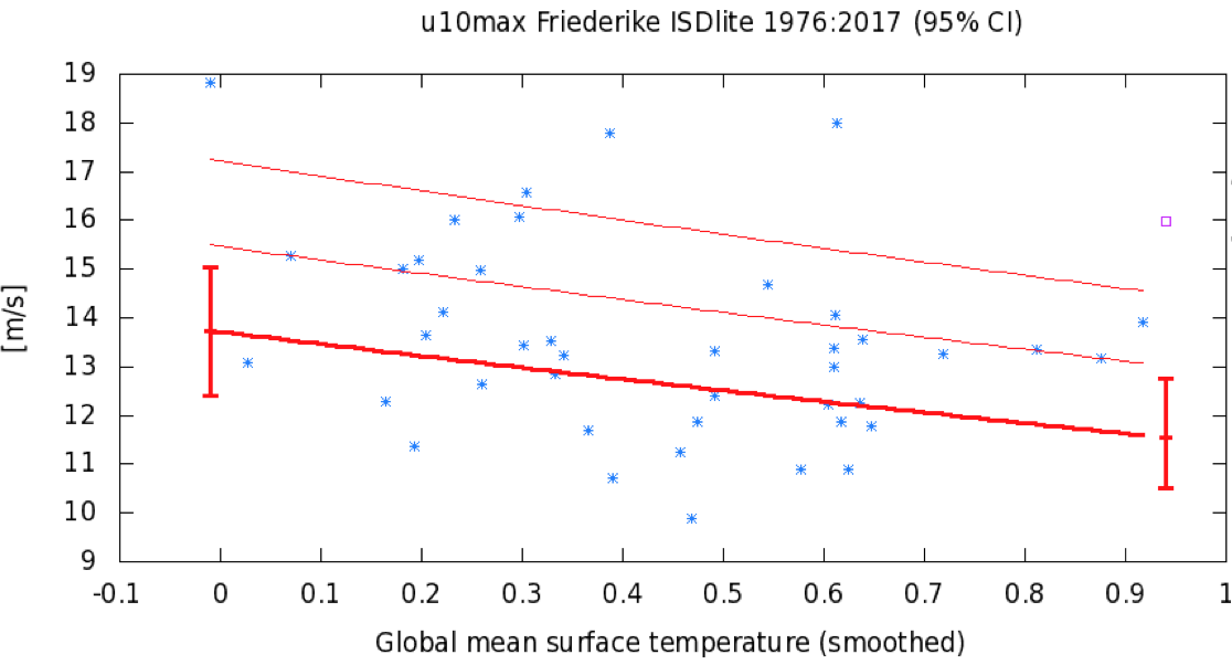
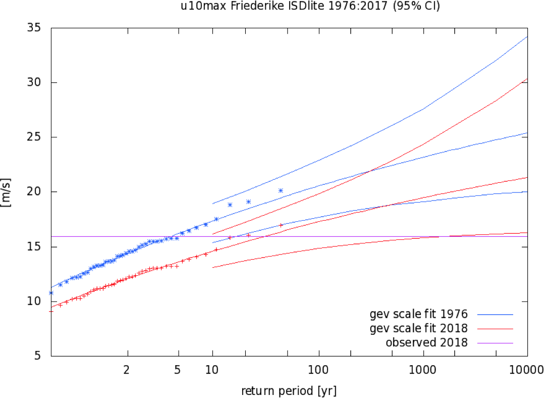
The winter maximum of the daily maximum of three-hourly maximum wind over the ISD-lite spatial average (over all stations in the box) is shown in Fig. 4a as a function of time (labeled with the year of the second half of winter). The data has been fitted by a GEV distribution in which the position parameter μ and scale parameter σ scale exponentially with time, such that their ratio remains constant. The shape parameter ξ is not time-dependent. We checked whether these assumptions are valid in the models, which have enough data not to need these assumptions. This fit shows a significant decrease (p<0.05 two-sided) in wind speed over 1976–2017, in agreement with earlier analyses (Smits et al, 2005, Vautard et al, 2010). The decrease in intensity of about 12% (95% CI 0–30%) corresponds to a decrease in probability of about a factor of four (95% CI: 1 to 100). Using the global mean temperature as a covariate instead of time gives slightly higher trends. The shape parameter ξ of the GEV is most likely negative, so the distribution has a tail that is thinner than a logarithmic function, so that the ratio of probabilities is more different from one for stronger storms.
The return period of an event like Friederike or worse in the area in which the indicator value reached 16.0 m/s on January 18 in the current climate is of the order of 20 years. In the 1970s, this was roughly five years, so the event has become a fairly rare event due to the decrease in high wind speeds observed during this period.
The result is confirmed in a different dataset from KNMI observations, with most stations showing a clear downward trend over the whole period (1971–2017 for two stations, 1982–2017 for most others, at least 30 years with data) of −15% [−7% to −17%], the same as the ISD-lite data show.. The trends are much less clear when starting in 1990 (using stations with at least 25 years of data). The trends in potential wind are much smaller (around −5%) and not statistically significant, even when pooled over all stations.
RACMO ensemble
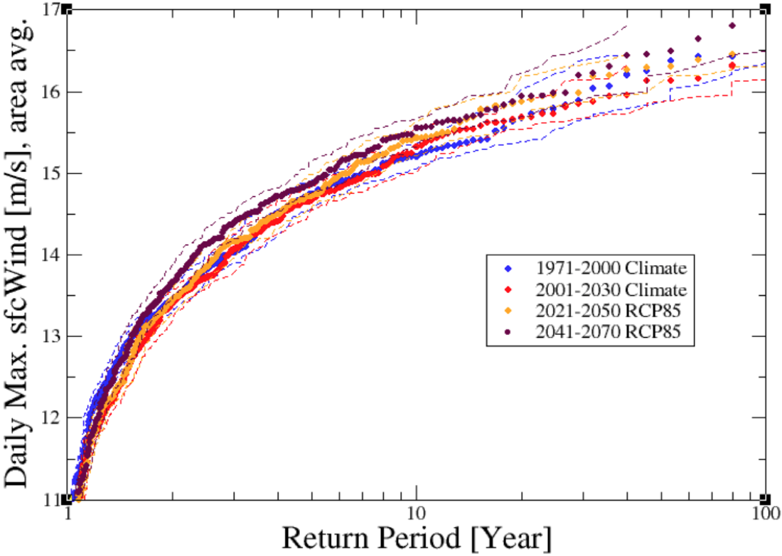
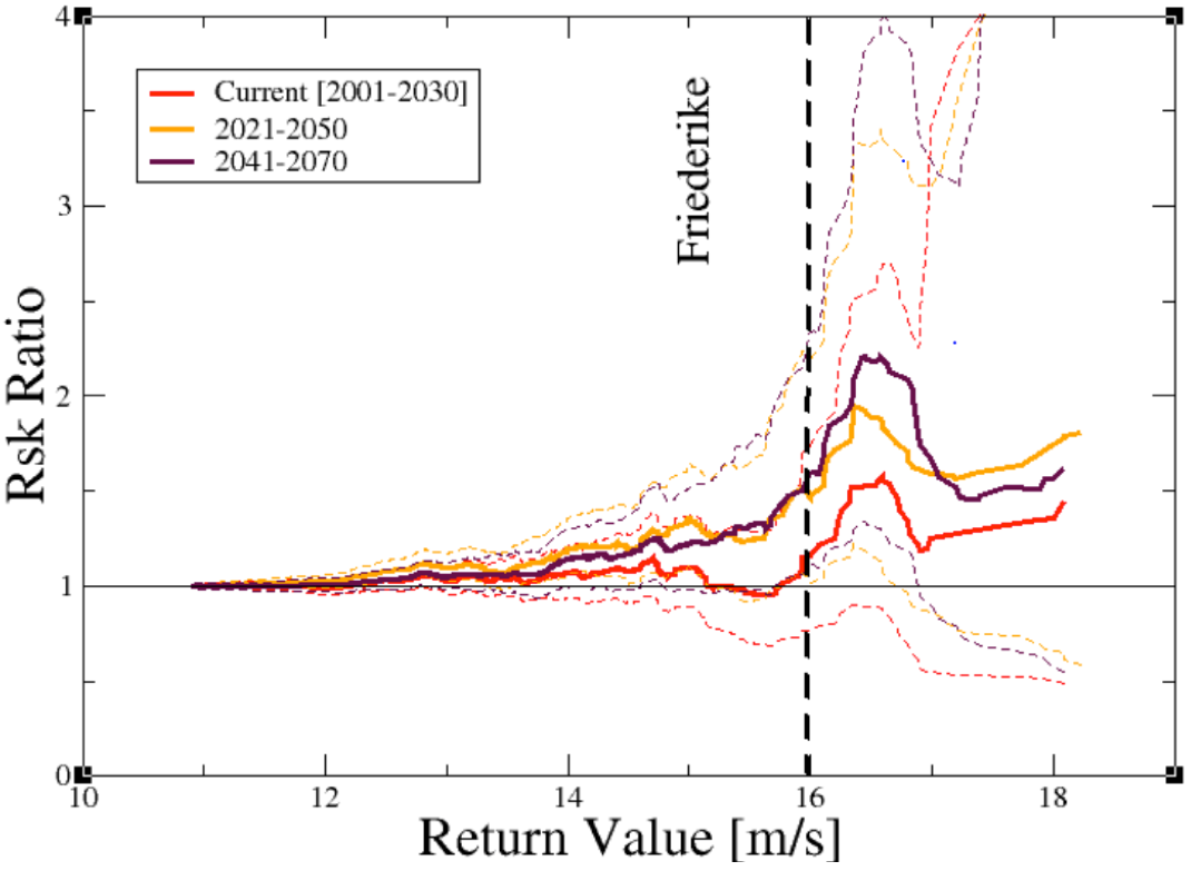
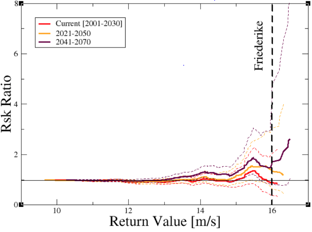
The RACMO ensemble is now pooled and the indicator is calculated from the simulations. The indicator is scaled to have the same 99th centile as the observed indicator in the historical period. Indicator statistics are then obtained for three climate periods: 1951-1980, simulating the “past” period, the “current” period taken as 2001-2030, and two future periods assuming the RCP8.5 scenario (2021-2050 and 2041-2060). The observed indicator value for storm Friederike (16.0 m/s) has a present return period of about 13 years (95% CI 10-19 years), which is longer than for the observations. The probability of witnessing higher indicator values is not significantly different in past and current periods (Figure 5). However, the change of probability becomes larger in future periods, with a risk ratio (RR) of about 1.5 [1-2] in the near term (Figure 5b). For this particular case, the increase is also stronger for stronger storms due to an increase in the variability relative to the mean.
Therefore, according to this model’s representation, we do not identify a climate change impact currently, but the increase in probability of storms like Friederike emerges in the coming decades. A fit with a GEV that scales with the global mean temperature of the driving EC-Earth ensemble gives no change (RR between 0.95 and 1.16), overlapping with the 30-year time window analysis (not shown), but this does not include the increase of variability relative to the mean.
HadGEM3A ensemble
The HadGEM3-A ensemble exhibits a significant difference between actual and counterfactual periods, with a current increase of strong daily mean winds in the area struck by Storm Friederike. However, due to the use of the mean wind speed instead of the maximum wind speed, the indicator does not disentangle extreme winds over a short time period from less strong winds over an extended time period. Accordingly, the observed value is not exceptional, due to the fast travelling nature of the extremely high winds in the area: for the value corresponding to Friederike (8.7 m/s), such events occur almost every year in both types of simulations. Note that difference in counterfactual and actual ensembles captures some changes in roughness, but probably not all.
EURO-CORDEX ensemble
In the EURO-CORDEX simulations, the return period corresponding to the scaled indicator (25-40 years) is larger, making it a more extreme event. The shape of the distribution is clearly different from that of the RACMO simulations and that of the observations (compare with Figs. 4 and 5). The RR is generally not significantly different from one (Figure 7b), despite a rather systematic increase. Such increase becomes marginally significant in the middle of the century with RR values in the range 1 to 3 for lower wind thresholds. Again, this indicates a tendency for more storms like Friederike in the future with a signal emergence not yet achieved. The GEV with smoothed EC-Earth global mean temperature as covariate confirms this conclusion, with an increase in probability of 1.0 to 1.2 (p~0.1), this corresponds to the assumption the percentage increase is a constant 0.0 to 1.4% per degree global warming over the whole range of Fig. 7a. This assumption holds well over the four 30-year time periods considered before.
Weather@Home
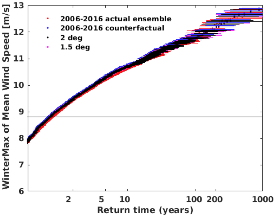
For weather@home, using the suboptimal definition of maximum of daily mean wind to define Storm Friederike (8.7 m/s), we find no significant change in the likelihood of storms like Friederike to occur (Figure 8). In contrast to the EURO-CORDEX assessment this also holds for rarer events (not shown).
| Ensemble | Ret. Period yr | RR for Current climate | RR for period 2021-2050 | RR for period 2041-2070 | RR for period PI+1.5°C | RR for period PI+2.0°C |
|---|---|---|---|---|---|---|
| Obs. ISD-Lite | N/A | N/A | N/A | N/A | ||
| Models using wind speed daily maximum (over 3 hourly data) | ||||||
| RACMO | 15 [11-19] | 1.1[0.8-1.7] | 1.5[1.0-2.2] | 1.5[1.1-2.3] | / | / |
| EURO-CORDEX | 40 [25-80] | 0.9[0.4-2.0] | 1.4[0.7-3.0] | 1.6[0.8-4.1] | / | / |
| Models using wind speed daily mean | ||||||
| HadGEM3-A | 1.2 [1.15-1.27] | 1.02 [0.98-1.06] | / | / | / | / |
| weather@home | 1.3[1.29-1.35] | 1.03[0.97-0.2] | / | / | 1.039[0.98-1.16] | 1.04[0.98-1.17] |
Table 2: Event return periods and risk ratios summarized for all model ensembles and for Storm Friederike. Risk ratios (RRs) are calculated with respect to a past or counterfactual period.
Storm Eleanor
Observations
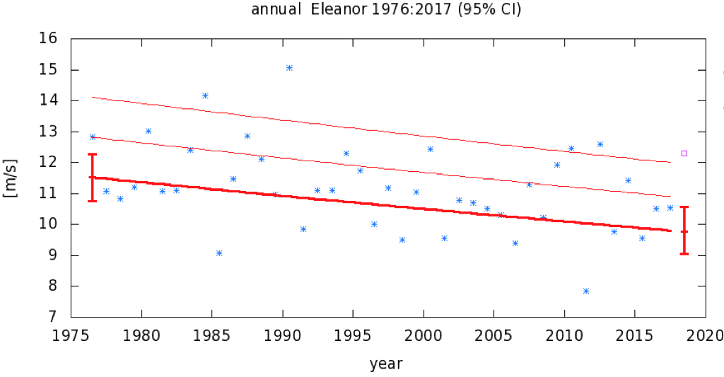
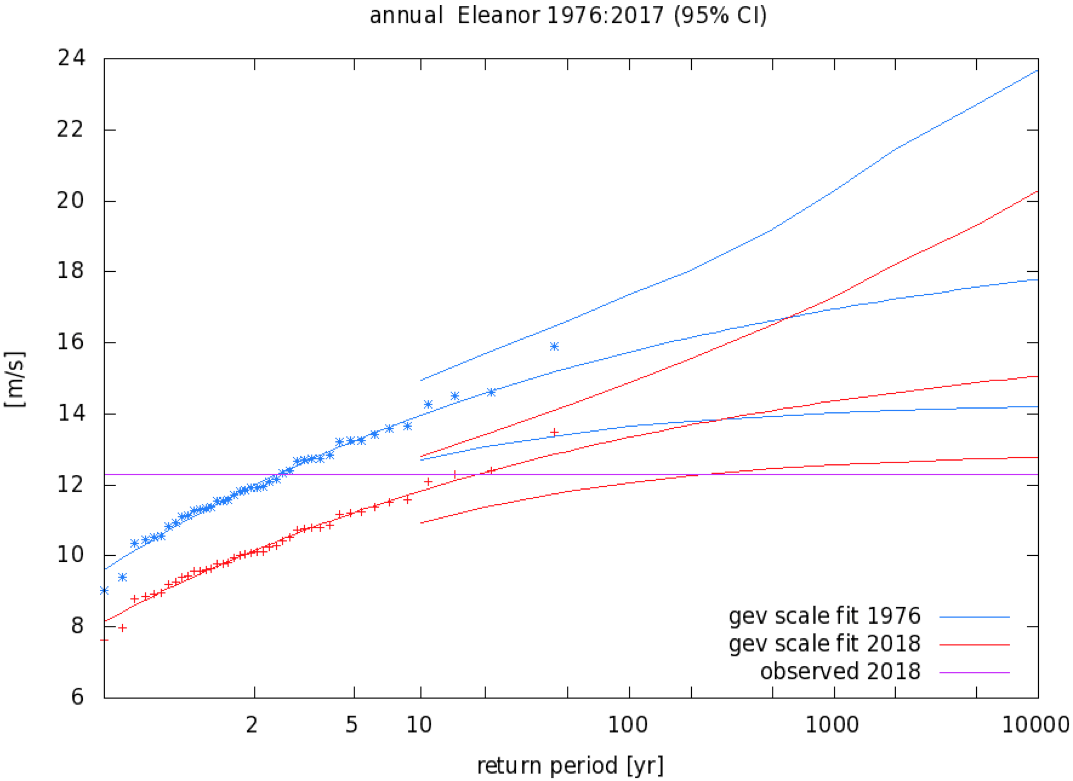
The same analysis on the Eleanor index as in section 4.1 gives a more significant downward trend for this storm (p<0.01 two-sided), with a decrease of about 20% (3–35%) (Figure 9). This corresponds to an increase in return period of a factor 8 (1.5–100). The return time also is about 20 years in the current climate according to this fit.
RACMO ensemble
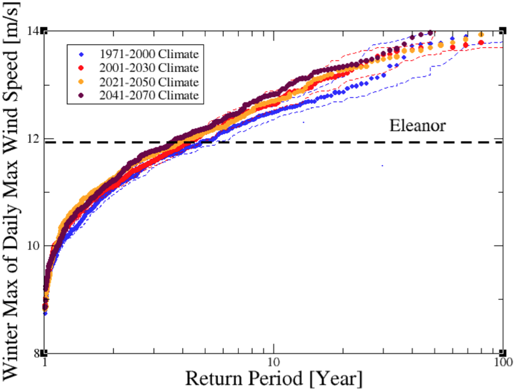
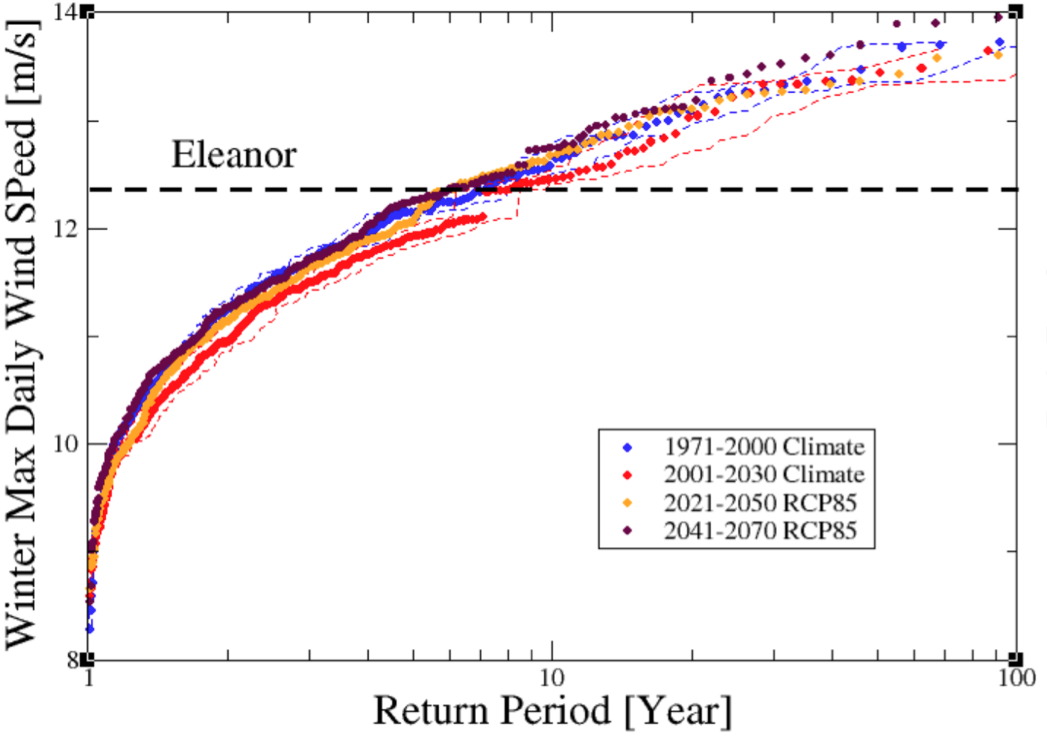
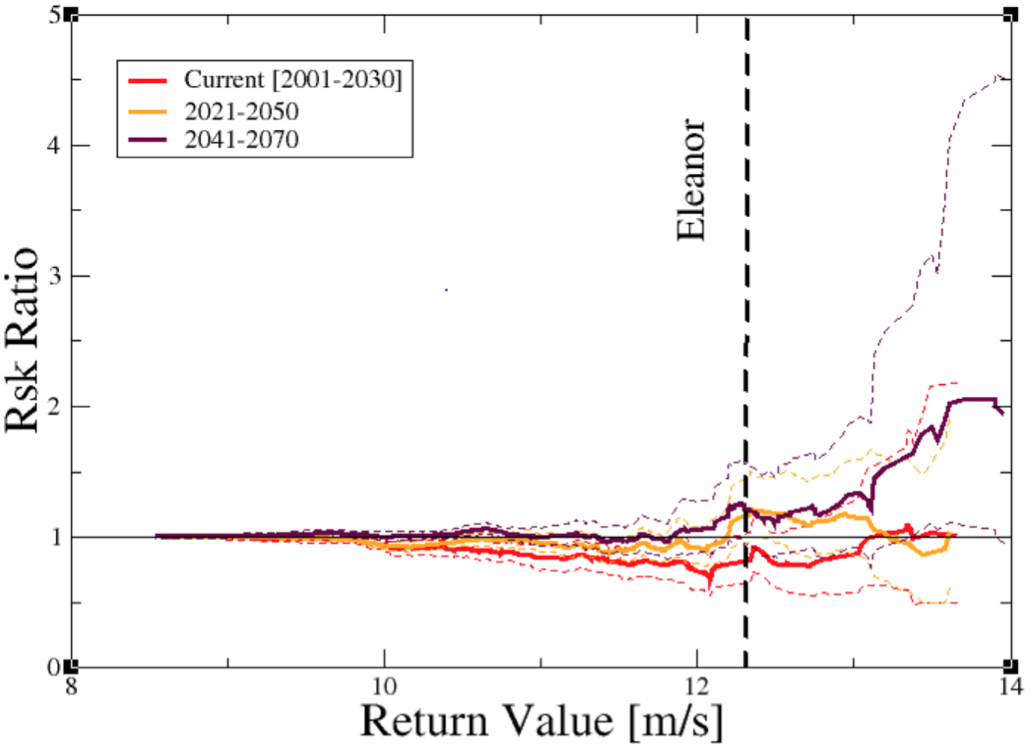
Storm Eleanor is now investigated through the wind daily maximum indicator with an average over the large region as defined above. Due to the southern boundary that is excluding a small band of the large region, we used for this model a boundary at 43.5N instead of 42N. This makes the indicator return value for stations slightly lower than when calculated over the full region (11.9 m/s instead of 12.3 m/s). The corresponding RACMO return period is in the range 3 to 5 years. The climate change is not significant for the current period and marginally significant for future periods, as for Storm Friederike (Figure 10). The estimated RR is 1.1 and slightly higher for future periods. Interestingly, for stronger storms, the RR increases. The same results hold for a GEV fit with covariate of all data in 1971-2070, with a RR significantly different from one (95% CI 1.0 to 1.2, not shown).
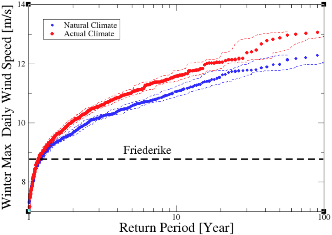
HadGEM3A ensemble
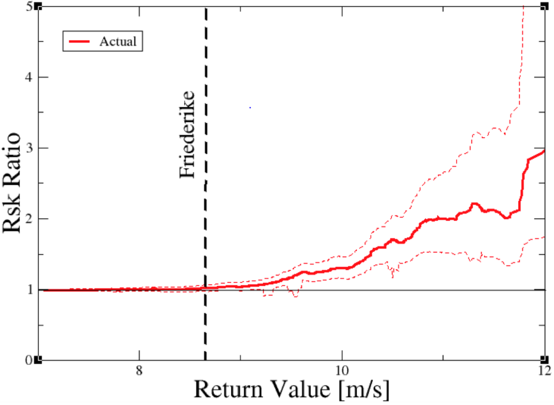
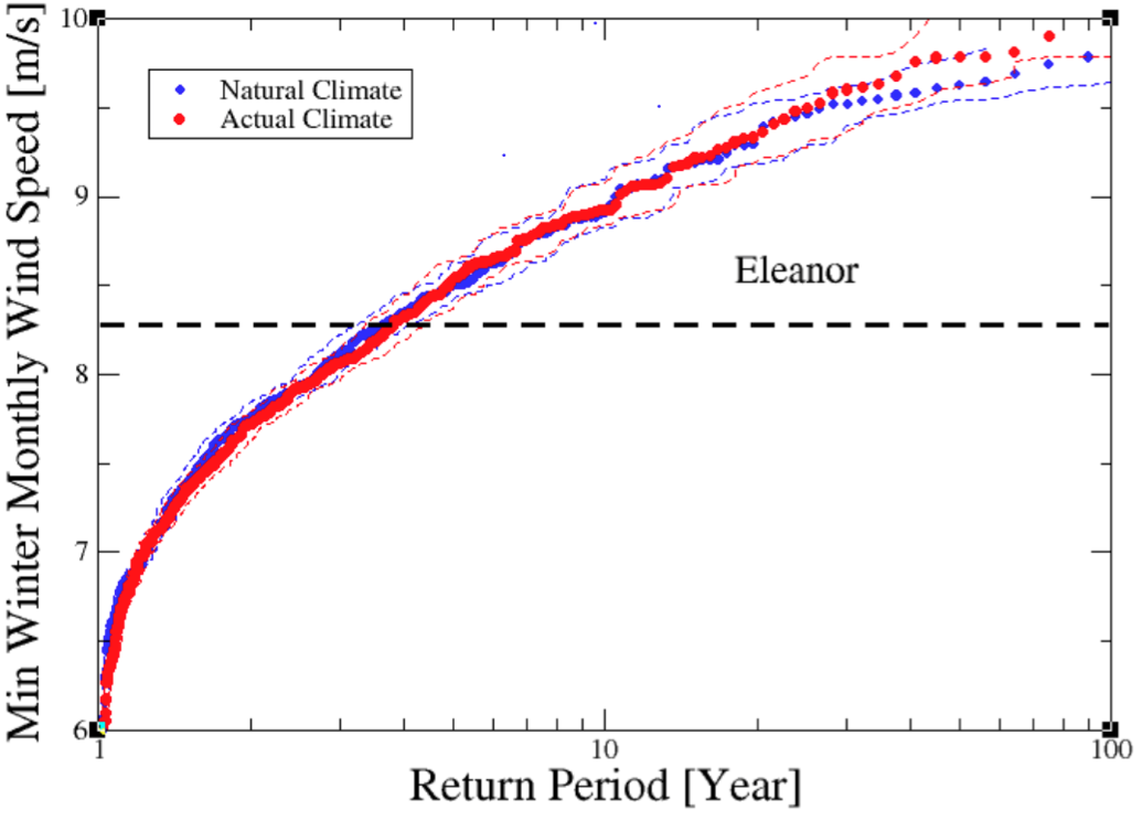
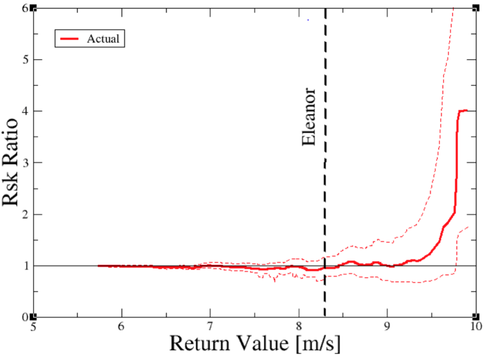
For HadGEM3-A, using the daily mean wind, we find no climate change signal in the estimation of the probabilities of high winds of any magnitude, but for the very extreme winds, we find marginally significant changes in the direction of more frequent high winds under current conditions than under natural conditions (Figure 11). The estimated return period for the indicator value corresponding to Eleanor, which does not fall in the extreme tail, lies also between three and five years. A risk ratio close to one is estimated.
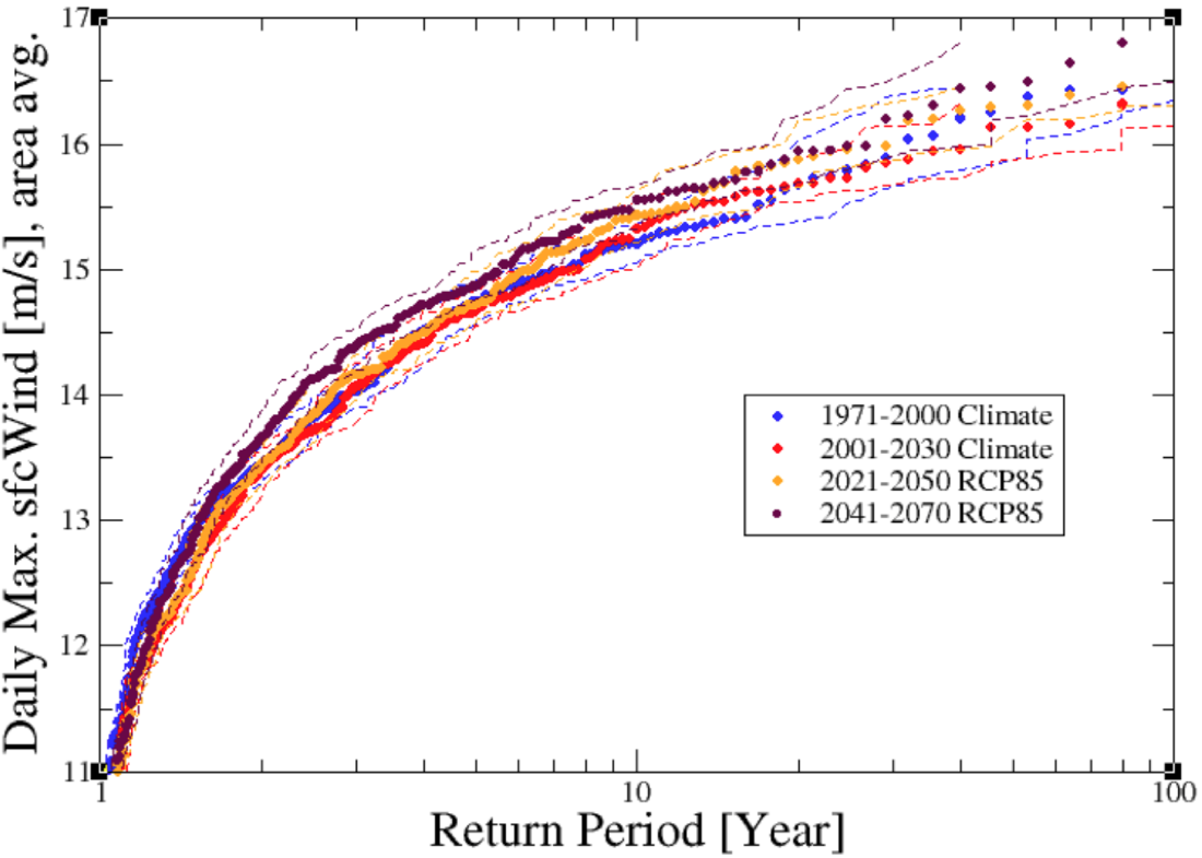
EURO-CORDEX ensemble
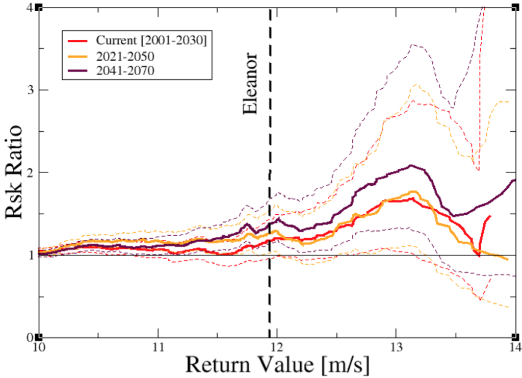
Using the EURO-CORDEX ensemble, the return period of the large-scale Storm Eleanor, characterized by the chosen indicator, is estimated to about 7-10 years. A climate change signal is absent in the simulations when comparing 1971-2000 and 2001-2030 periods. For the indicator value, the RR is in the range [0.5-1]. Only for later periods and for larger indicator values, a marginally significant increase in the RR in the range [1-2] can be seen (Figure 12). A GEV with a modelled global mean temperature (from EC-Earth) as covariate also gives a non-significant increase with a RR between 0.99 and 1.15 (95% CI).
Weather@Home
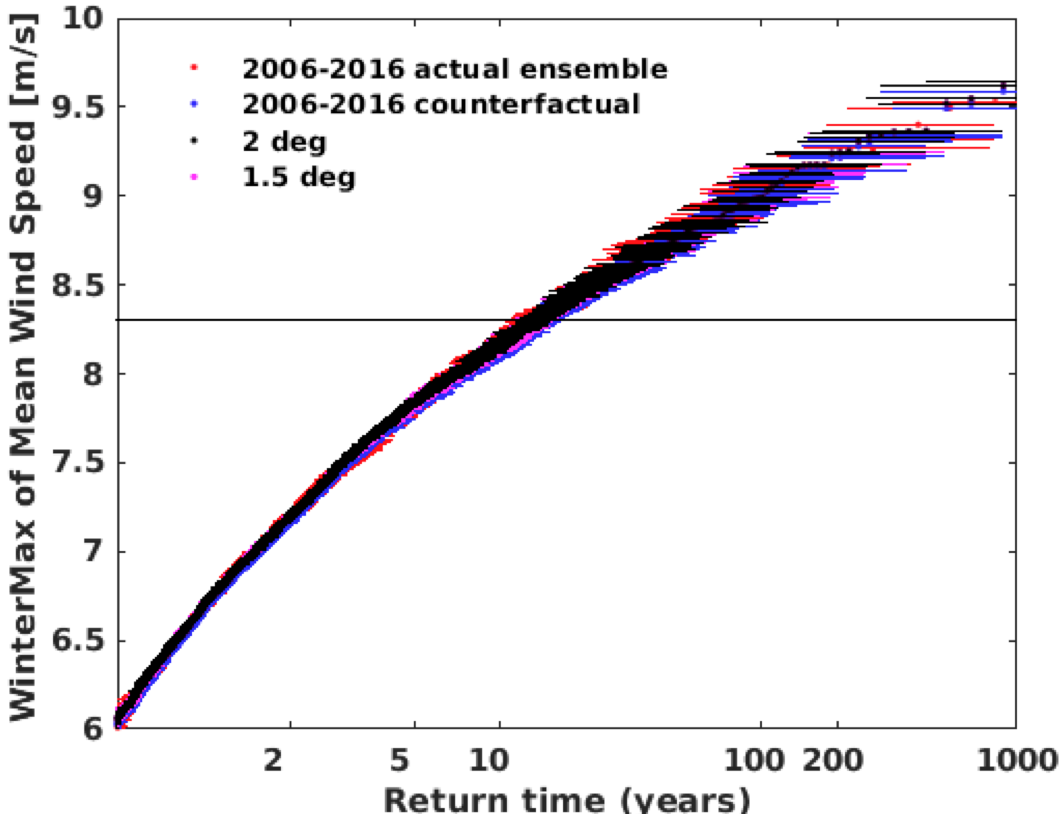
For weather@home, using the maximum of daily mean wind to define Storm Eleanor (8.3 m/s), we find no significant change in the likelihood of storms like Eleanor to occur. In contrast to the EURO-CORDEX assessment, this also holds for rarer events where the weather@home model shows a non-significant decrease in high wind speeds.
| Ensemble | Ret. Period yr | RR for Current climate | RR for period 2021-2050 | RR for period 2041-2070 | RR for period PI+1.5°C | RR for period PI+2.0°C |
|---|---|---|---|---|---|---|
| Obs. ISD-Lite | N/A | N/A | ||||
| RACMO | 4.2[3.7-4.8] | 1.2[1.0-1.4] | 1.3[1.0-1.5] | 1.3[1.1-1.6] | / | / |
| HadGEM3-A | 3.9[3.4-4.5] | 1.0[0.8-1.2] | / | / | / | / |
| EURO-CORDEX | 6.6 [5.6-6.9] | 0.8[0.6-1.0] | 1.2[1.-1.4] | 1.2[0.9-1.6] | / | / |
| weather@home | 13.9[13.6-15] | 1.01[0.62-2.35] | / | / | 0.94[0.6-2.35] | 0.94[0.59-2.36] |
Table 3: Event return periods and risk ratios summarized for all model ensembles and for Storm Eleanor.
Synthesis and conclusions
Western European countries have been struck by high-impact wind storms during the month of January 2018. The link between storms like Eleanor (on 3/1/2018) and Friederike (on 18/1/2018) and climate change have been studied through this attribution analysis involving several simulation ensembles and observations from tens of weather stations.
From an analysis of two sets of observations, we conclude that near-surface storms in the areas of the two storms have a decreasing trend in wind speed and, hence, frequency trend over the past 40 years (see Figure 13), consistent with previous observation-based studies on storminess in these areas (Smits et al., 2005; Soubeyroux et al., 2017) and with global land wind stilling (Vautard et al., 2010; McVicar et al., 2012). This trend was shown to be close to zero over the Netherlands area when using the potential wind, showing a strong influence of roughness changes there (see also Wever, 2012). Other processes, such as aerosols increase, could also induce a wind decrease (Bichet et al., 2012), and decadal-scale long-term variability has been shown to have a significant role as well (e.g., Matulla et al, 2008).
We next turn to the model results. Due to the differing experiments that we used, the risk ratios have been computed over different intervals. To compare those we need to convert them to a common interval. We do this by assuming the risk ratio is an exponential function of some indicator of global warming f(yr):
RR(y1,yend) = RR(y2,yrend) RR(yr1,yr2) = RR(yr2,yrend) exp[f(yr1)-f(yr2)]
In the following, we use the RCP4.5 CO2 concentration for f(yr), as the global mean temperature has no observations in the future and the projections depend on the model.
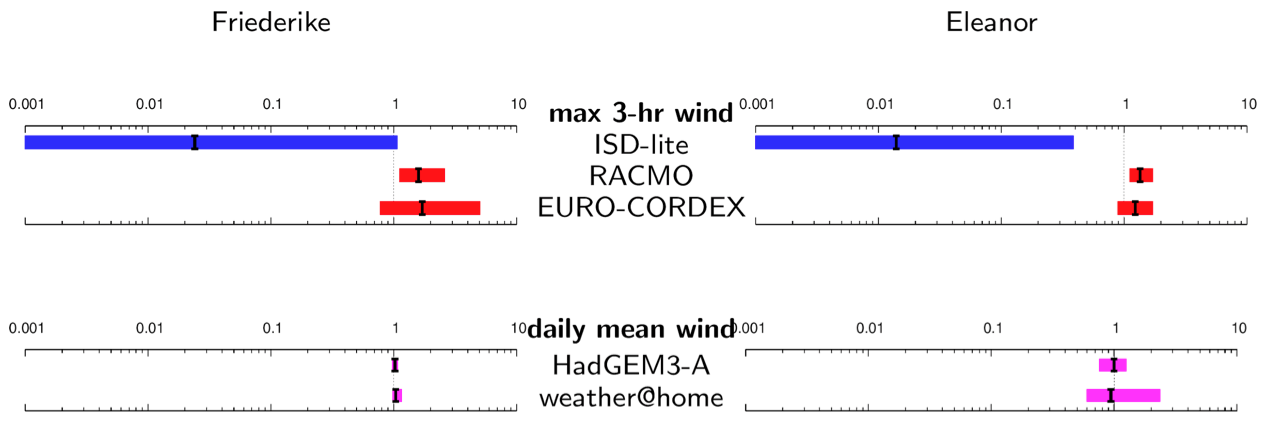
In contrast to the observations, global and regional climate models do not simulate such a decrease over the past decades. Instead, simulations of the daily maximum of 3-hourly instantaneous wind, of the same spatial and temporal characteristics of these storms and, hence, the observational analysis, indicate increases in probability between 1975 and 2055, corresponding to increases in wind speed for this return time. These are not all significantly different from one, but model consensus and future trends support the presence of such positive tendency. The change is small though: a risk ratio of 1.5 for Friederike with an uncertainty range of 1 to 2, corresponding with an increase in intensity of the wind of only about 5% (0% to 10%). For Eleanor, the numbers are even smaller: an increase in RR of about 1.25 (1.0 to 1.6) or an increase in intensity of 2% (0% to 5%).
The changes in daily mean wind are smaller still and indistinguishable from no change. However, as these do not correspond directly to the impact of these storms, we do not take them into account in the synthesis.
The climate model simulations do not always include changes in aerosols and either have no roughness changes (regional models) or capture these only partially (HadGEM3-A). This explains at least partially the conflict with the observed trends, as the potential wind results for the Netherlands showed that roughness plays a large role in the observed decrease in storminess. By contrast, these model ensembles mainly reflect changes due to greenhouse gases.
We conclude that storms like Friederike and Eleanor have not become significantly more or less frequent due to climate change, but our model results indicate that global warming due to greenhouse gases could make storms like them somewhat more frequent in the future, with a frequency increase up to at most a factor of two, or equivalently a few percent higher wind speeds. However, the observations show a clear decline in high wind speeds, in accordance with earlier studies. This is equivalent to declining probabilities of these kind of storms, but our analysis and previous studies find explanations for these changes in factors other than greenhouse gases. The increase in roughness potentially explains a major part of this decrease, and does not exclude other factors, such as decadal variability and aerosol effects. Until a quantitative attribution of past observed decreases is established, and with that an understanding of the interplay between greenhouse gas forcing and those other factors, and scenarios for them, the confidence on future evolutions of wind storms will remain low, based on simulations reflecting mainly the effects of greenhouse gas increases.
Acknowledgements
This work was supported by the EUPHEME project, which is part of ERA4CS, an ERA-NET initiated by JPI Climate and co-funded by the European Union (Grant #690462). It was also supported by the French Ministry for an Ecological and Solidary Transition through national convention on climate services. We would like to thank all volunteers who have donated their computing time to weather@home.
References
Aalbers, E.E., G. Lenderink, E. van Meijgaard, B.J.J.M. van den Hurk (2017). Local-scale changes in mean and heavy precipitation in Western Europe: climate change or internal variability? Climate Dynamics, 50 (11–12): 4745–4766. doi: 10.1007/s00382-017-3901-9
Bichet, A., Wild, M., Folini, D., & Schär, C. (2012). Causes for decadal variations of wind speed over land: Sensitivity studies with a global climate model. Geophysical Research Letters, 39(11). doi: 10.1029/2012GL051685
Christidis, N., Stott, P. A., Scaife, A. A., Arribas, A., Jones, G. S., Copsey, D., … & Tennant, W. J. (2013). A new HadGEM3-A-based system for attribution of weather-and climate-related extreme events. Journal of Climate, 26(9): 2756-2783. doi: 10.1175/JCLI-D-12-00169.1
Lenderink, G., B.J.J.M. van den Hurk, A.M.G. Klein Tank, G.J. van Oldenborgh, E. van Meijgaard, H. de Vries and J.J. Beersma (2014). Preparing local climate change scenarios for the Netherlands using resampling of climate model output. Environmental Research Letters, 9(11): 115008. doi: 10.1088/1748-9326/9/11/115008
Matulla, C., Schöner, W., Alexandersson, H., von Storch, H. (2008). European storminess: late nineteenth century to present. Climate Dynamics, 31: 125–130. doi: 10.1007/s00382-007-0333-y
McVicar, T. R., Roderick, M. L., Donohue, R. J., Li, L. T., Van Niel, T. G., Thomas, A., Grieser, J., Jhajharia, D., Himri, Y., Mahowald, N.M., Mescherskaya, A.V.,Kruger, A.C., Rehman, S. and Dinpashoh, Y. (2012). Global review and synthesis of trends in observed terrestrial near-surface wind speeds: Implications for evaporation. Journal of Hydrology, 416: 182-205. doi: 10.1016/j.jhydrol.2011.10.024
Michelangeli, P.A., Vautard, R., Legras, B. (1995). Weather regimes: recurrence and quasi-stationarity. Journal of Atmospheric Science, 52: 1237-1256. doi: 10.1175/1520-0469(1995)052<1237:WRRAQS>2.0.CO;2
Philip, S., S. F. Kew, G. J. van Oldenborgh, E. Aalbers, R. Vautard, F. Otto, K. Haustein, F. Habets, R. Singh and H. Cullen (2018). Validation of a rapid attribution of the May/June 2016 flood-inducing precipitation in France to climate change. Climate Dynamics, in preparation. doi: 10.1175/JHM-D-18-0074.1
Schaller, N., A.L. Kay, R. Lamb, N.R. Massey, G.-J. van Oldenborgh, F.E.L. Otto, S.N. Sparrow, R. Vautard, P. Yiou, A. Bowery, S.M. Crooks, C. Huntingford, W. Ingram, R. Jones, T. Legg, J. Miller, J. Skeggs, D. Wallom, S. Wilson & M.R. Allen. (2015). Human influence on climate in the 2014 Southern England winter floods and their impacts. Nature climate change, 6, pages 627–634 (2016). doi:10.1038/nclimate2927
Smits, A. A. K. T., Klein Tank, A. M. G., & Können, G. P. (2005). Trends in storminess over the Netherlands, 1962–2002. International Journal of Climatology, 25(10), 1331-1344. doi:10.1002/joc.1195
Soubeyroux, J.-M., Dosnon, F., Richon, J., Schneider, M., and P. Lassègues, (2017). Caractérisation à haute résolution spatiale des tempêtes historiques en métropole application à la tempête Zeus du 6 mars 2017. La Climatologie, 14.
Vautard, R., J. Cattiaux, P. Yiou, J.-N Thepaut, and P. Ciais. (2010). Northern Hemisphere atmospheric stilling partly attributed to an increase in surface roughness. Nature Geoscience, 3: 756–761. doi: 10.1038/ngeo979
Vautard, R., A. Colette, E. van Meijgaard, F. Meleux, G. J. van Oldenborgh, F. Otto, I. Tobin, P. Yiou. (2017). Attribution of wintertime anticyclonic stagnation contributing to air pollution in Western Europe. Bulletin of American Meteorological Society, in Explaining extreme events of 2016 from a climate perspective, special supplement, S70-S75. doi: 10.1175/BAMS-D-17-0113.1
Vautard, R., N. Christidis, A. Ciavarella, C. Alvarez-Castro, O. Bellprat, B. Christiansen, I. Colfescu, T. Cowan, F. Doblas-Reyes, J. Eden, M. Hauser, G. Hegerl, N. Hempelmann, K. Klehmet, F. Lott, C. Nangini, R. Orth, S. Radanovics, S. I. Seneviratne, G. J. van Oldenborgh, P. Stott, S. Tett, L. Wilcox, P. Yiou (2017). Evaluation of the HadGEM3-A simulations in view of climate and weather event human influence attribution in Europe. Climate Dynamics, submitted. doi: 10.1007/s00382-018-4183-6
Vrac, M., Noël, T. and R. Vautard. (2016). Bias correction of precipitation through Singularity Stochastic Removal: Because occurrences matter. Journal of Geophysical Research, 121(10): 5237-5258. doi: 10.1002/2015JD024511
Weber, N. and G. Groen. (2009). Improving potential wind for extreme wind statistics, KNMI Scientific Report WR 2009-02.
Wever, N. (2012). Quantifying trends in surface roughness and the effect on surface wind speed observations. Journal of Geophysical Research: Atmospheres: 117(D11). doi: 10.1029/2011JD017118